
In this post I give an introduction to several generative models in deep learning literature, including adversarial networks (GANs), variational autoencoder (VAE) and flow models. I also derive the formula for evaluating flow densities on generated samples.
Deep generative models concern the problem of finding high dimensional data distribution, and new data generation. There are four major types of generative models in the literature: generative adversarial networks (GANs) [1], variational autoencoder (VAE) [2], normalizing flows [3,4,5], plus autoregressive models [6]. In all the first three models, the approach to data generation is to make use of some noise space, denoted as \(\mathcal{Z}\). A mapping from the noise space to data space is learned, using training data and various training methods. To obtain a sample from the generative model, one first samples a noise vector \(z\) from the noise space \(\mathcal{Z}\), and then inputs the noise vector to the learned mapping, and obtains generated sample from the model output. The intuition that why one should generate data from noise space via a learned mapping may come from the observation that for many common distributions like Gaussian, samples can be generated as a transformation of noises.
The three classes of models differ in interpretation of the noise space, model specification and learning methods. In GAN, a direct mapping from the noise space to data space is specified, where the noise space typically has smaller dimension than the data space. To train the model, one adds a classifier that discriminates between real and generated data, and jointly trains the two models through playing a minimax game. In VAE the mapping between noise space and data space is formulated in a probabilistic way, so that we can obtain the formula for likelihood on data. The likelihood is intractable to compute, so instead the model is trained by maximizing a lower bound on the log density. Flow models come with both exact likelihood evaluation as well as sample generation. Jacobians of the transformations between the two spaces are used to compute the likelihood.
We now discuss these three generative models in in some detail. We shall use the following notations: \(\mathcal{X}\) denotes data space, which is usually a subset of \(\mathbb{R}^d\) for some dimension \(d\). \(\mathcal{Z}\) denotes noise space, and \(Z\) denotes a generic random variable taking values in \(\mathcal{Z}\) with distribution \(p_Z\), for example a standard multivariate Gaussian.
 Three Classes of Generative Models
Generative Adversarial Networks
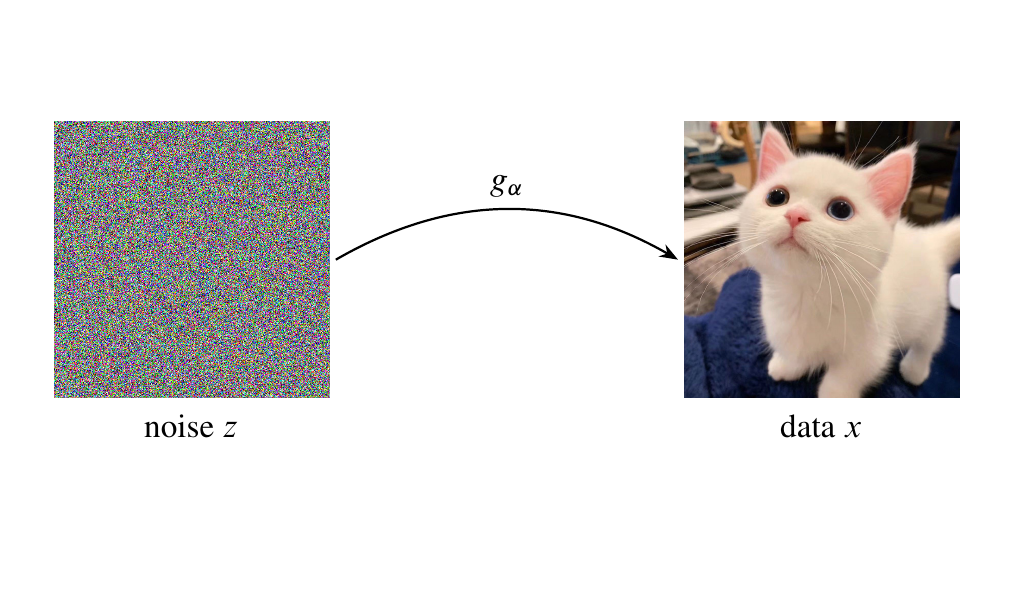
In GAN, a data generator \(g_\alpha\) from noise space to data space is specified:
\[\begin{gathered} g_\alpha: \mathcal{Z}\to \mathcal{X}\\ z\mapsto x \end{gathered}\]which is typically parametrized by neural networks. A simple distribution on \(\mathcal{Z}\), like a standard Gaussian \(p_Z\), is also specified. We would like to train the generator \(g_\alpha\) so that it transforms the distribution \(p_Z\) on \(\mathcal{Z}\) to the data distribution \(p_{\text{data}}\) on \(\mathcal{X}\) for as close as possible, i.e., given \(z\sim p_Z\), the output \(g_\alpha(z)\) should closely follow the data distribution. To achieve this goal, one adds a second discriminator
\[D_\theta: \mathcal{X} \to [0,1]\]that assigns its input a probability score indicating how likely it is from the true data distribution. If \(D_\theta(x)\) is close to \(1\) then it may classify \(x\) as coming from the true data distribution, while if \(D_\theta(x)\) is close to \(0\) then it may classify \(x\) as coming from the generator \(g_\alpha\). One then jointly trains the two model together by performing
\[\min_\alpha\max_\theta V(\alpha, \theta)\]with
We see that \(\max_\theta V(\alpha, \theta)\) means pushing up \(D_\theta\) on data manifold while pushing down \(D_\theta\) on generated output from \(g_\alpha\). On the other hand, \(\min V(\alpha, \theta)\) means finding \(\alpha\) so that \(g_\alpha(z)\) are located at places where \(D_\theta\) has large values, which should ideally be closer and closer to the true data distribution as training proceeds, from the update of \(D_\theta\) in \(\max_\theta V(\alpha, \theta)\) just mentioned.
Variational Autoencoders
A variational autoencoder consists of a probabilistic decoder \(p_\alpha(x\mid z)\) from latent space \(\mathcal{Z}\) to data space \(\mathcal{X}\), and a probabilistic encoder \(q_\phi(z\mid x)\) from \(\mathcal{X}\) to \(\mathcal{Z}\), both of which are parametrized by neural networks. Given \(z\) sampled from \(p_Z\), the decoder returns a conditional probability distribution \(p_\alpha(\cdot\mid z)\) on \(\mathcal{X}\). The unconditional density \(p_\alpha(x)\) is
\[p_\alpha(x) = \int p_\alpha(x\mid z)p_Z(z)dz\]One would like to use the above equation to perform maximum likelihood estimation on training data. However, the integral is intractable to compute. Instead, one has to use the encoder to obtain a tractable lower bound on the log density, and maximize the lower bound:
where the inequality is from Jensen’s inequality. To compute the lower bound \(\mathcal{L}_{\alpha,\phi}(x)\) on training data \(x^{(i)}\), we send the data to the encoder, to obtain a distribution \(q_\phi(z\mid x^{(i)})\) on \(\mathcal{Z}\). Then we can sample \(z\) from this distribution and feed \(z\) to the decoder network and evaluate the decoder distribution on \(x^{(i)}\). This is the first term \(\mathbb{E}_{z\sim q_\phi(z\mid x^{(i)})}\log p_\alpha(x^{(i)}\mid z)\) in \(\mathcal{L}_{\alpha,\phi}(x)\). We are also able to compute the KL divergence between \(q_\phi(z\mid x^{(i)})\) and the prior distribution \(p_Z(z)\) on \(\mathcal{Z}\), for example a standard Gaussian. Design choices of the decoder \(p_\alpha(x\mid z)\) depend on the type of data one is modeling. Common choice is to output multivariate Bernoulli for discrete data and multivariate Gaussian for continuous data. The prior distribution \(p_Z\) as well as the encoder \(q_\phi(z\mid x)\), however, should be assumed to be continuous. The reason is explained below.
To compute the gradient of \(\mathcal{L}_{\alpha,\phi}(x)\) with respect to \(\phi\), we have to differentiate through an expectation on the latent variables. We can use a technique called the reparameterization trick to avoid computing the integral of the expectation. We first describe it in general terms, then apply it to the current case.
Given a random variable \(X\) with density \(q_\alpha\), where \(\alpha\) is some set of parameters, and a scalar function \(f\), the problem is to compute the gradient of the expectation of \(f\) with respect to \(\alpha\):
\[\nabla_\alpha \mathbb{E}_{x\sim q_\alpha}f(x) = \nabla_\alpha \int f(x)q_\alpha(x)dx.\]\(f\) may or may not depend on parameter \(\alpha\), but for simplicity we assume it doesn’t. If \(X\) can be expressed as a differentiable transformation of random variable \(Z\) with simple density \(p_Z\), for example a Gaussian or uniform distribution:
\[x = g_\alpha(z)\quad \text{for some }z\sim p_Z,\]then we are able to move the expectation operation out:
\[\begin{split} \nabla_\alpha \mathbb{E}_{x\sim q_\alpha}f(x) &= \nabla_\alpha \mathbb{E}_{z\sim p_Z}f(g_\alpha(z))\\ &= \mathbb{E}_{z\sim p_Z}\nabla_\alpha f(g_\alpha(z)). \end{split}\]In particular, when we have finite samples \(\{x_\alpha^{(1)},\ldots,x_\alpha^{(N)}\}\) from \(q_\alpha\), and we’d like to compute \(\nabla_\alpha\frac{1}{N}\sum_{i=1}^Nf\left(x_\alpha^{(i)}\right),\) we can take the random numbers \(\{z^{(1)},\ldots,z^{(N)}\}\) that are used to generate the samples, and compute \(\nabla_\alpha\frac{1}{N}\sum_{i=1}^Nf\left(g_\alpha\left(z^{(i)}\right)\right).\) An example is when \(q_\alpha\) is Gaussian with some mean \(\mu_\alpha\) and variance \(\sigma_\alpha\) that are both some closed-form functions of the parameter \(\alpha\). In this case \(g_\alpha\) is simply an affine transformation of standard Gaussian:
\[g_\alpha(z) = \mu_\alpha + \sigma_\alpha\cdot z \quad\text{where } z\sim \mathcal{N}(0,I)\]and the gradient computation becomes
\[\nabla_\alpha\frac{1}{N}\sum_{i=1}^Nf\left(\mu_\alpha + z^{(i)}\cdot \sigma_\alpha\right).\]In VAE, the prior distribution of latent space \(p_Z\) is often assumed to be standard Gaussian, and in the training process the aim is to match the encoder network \(q_\phi(z\mid x)\) to this prior for as much as possible. In view of the reparameterization trick explained above, we can directly formulate the encoder network \(q_\phi(z\mid x)\) as \(\mu_\phi(x)\) and \(\sigma_\phi(x)\) where they both can be some complicated nonlinear transformation of the input, for example fully connected neural networks. To sample noise/latent variable \(z\) from \(q_\phi(z\mid x)\), we simply sample \(\epsilon\sim \mathcal{N}(0,I)\) and transform the noise as
\[z = \mu_\phi(x) + \epsilon\cdot\sigma_\phi(x).\]Then we can feed the \(z\) to the objective \(\log p(x\mid z)\). In particular, we can write the gradient of the the first term with respect to \(\phi\) in the lower bound on training data \(\{x^{(1)},\ldots,x^{(N)}\}\) as
\[\nabla_\phi\frac{1}{N}\sum_{i=1}^N\log p_\alpha\left(x^{(i)}\mid \mu_\phi(x^{(i)}) + \epsilon_i\cdot\sigma_\phi(x^{(i)})\right).\]The reparameterization trick works only if the distribution with respect to which we are differentiating can be expressed as a differentiable (and in particular, continuous) transformation of simple noise distributions. In case the distribution is discrete, it is not possible to express the samples as such differentiable transformations, and one has to rely on other techniques.
Normalizing Flows
A normalizing flow model is an invertible mapping from data space to a noise space with the same dimensionality:
\[\begin{gathered} f_\alpha: \mathcal{X} \to \mathcal{Z}\\ x \mapsto z, \end{gathered}\]together with a simple distribution \(p_Z\) on \(\mathcal{Z}\) like a standard Gaussian. To sample from the model, one first samples from the noise distribution \(z\sim p_Z\) and invert the mapping to obtain \(\tilde{x}=f^{-1}_\alpha(z)\). The distinct characteristic of flow models is that one can leverage the change of variable formula for probability distributions to obtain exact likelihood evaluation \(p_\alpha(x)\) on \(\mathcal{X}\):
\[p_\alpha(x) = p_Z(f_\alpha(x))\cdot\left|\frac{\partial}{\partial x}f_\alpha(x)\right|,\]or
\[\log p_\alpha(x) = \log p_Z(f_\alpha(x))+ \log\left|\frac{\partial}{\partial x}f_\alpha(x)\right|,\]where \(\left\lvert\frac{\partial}{\partial x}f_\alpha(x)\right\rvert\) denotes the absolute value of the determinant of the Jacobian of the transformation \(f_\alpha\) at point \(x\in\mathcal{X}\). Since we have exact log-likelihood, we can use MLE to train the model. One chooses the invertible transformation \(f_\alpha\) in such a way that this log determinant of Jacobian is easy to compute. Recall that if a square matrix \(A\) is triangular, then \(\det(A)\) is the product of the elements along the diagonal, so \(\log\lvert\det(A)\rvert\) is simply the summation of its diagonal entries after the log function is applied element-wise. Thus, one way to design a flow model is to use some basic transformations \(h_{\alpha_1},\ldots,h_{\alpha_m}\) as building blocks, all of which have such triangular Jacobian matrices, and compose them together to obtain the model as
\[f_\alpha = h_{\alpha_m}\circ\cdots\circ h_{\alpha_1}.\]To compute model output \(\log p_\alpha(x)\), we map \(x\) through all the transformations to \(f_\alpha(x)\), evaluate \(p_Z\) at \(f_\alpha(x)\), then add all log absolute determinant of Jacobians of all transformations.
Examples of flow model include NICE [3], Real NVP [4], and Glow [5]. The basic building block of such model is the affine coupling layer. For an input \(x=(x_1,\ldots,x_d)\) with dimension \(d\), the output of the affine coupling layer \(y=(y_1,\ldots,y_d)\) is
\[\begin{cases} y_{1:d'} = x_{1:d'},\\[0.2cm] y_{d'+1:d} = x_{d'+1:d} \odot s(x_{1:d'}) + t(x_{1:d'}) \end{cases}\]where \(d'<d\). \(s(\cdot)\) is the scale function and \(t(\cdot)\) is the translation function, both of which can be complex transformation of their inputs, for example fully connected neural networks or convolutional neural networks. The Jacobian of the transformation is lower-triangular:
\[\frac{\partial y}{\partial x^T} = \begin{pmatrix} I_{d'} & 0 \\[0.2cm] * & \mathrm{diag}(s(x_{1:d'}))\end{pmatrix}\]where \(*\) is the part that is not relevant for density calculation, and \(\mathrm{diag}(s(x_{1:d'}))\) is the diagonal matrix whose diagonal vector is \(s(x_{1:d'})\). We see that the log determinant of the affine coupling transformation is simply \(\texttt{sum}(\log\lvert s\rvert)\), namely we just need to apply absolute value and the the log function element-wise, and then sum the result. The transformation is also easily invertible:
\[\begin{cases} x_{1:d'} = y_{1:d'},\\[0.2cm] x_{d'+1:d} = (y_{d'+1:d} - t(x_{1:d'})) \odot s^{-1}(x_{1:d'}). \end{cases}\] Affine Coupling Layer
Autoregressive flows
Autoregressive flow models [7,8,9] can be seen as a specific class of normalizing flows. In autoregressive flow, an input data \(x=(x_1,x_2,\ldots,x_d)\in\mathbb{R}^d\) is mapped to the output noise \(z=(z_1,z_2,\ldots,z_d)\in\mathbb{R}^d\) through the following structure:
\[\begin{aligned} z_1 &= f_\alpha(x_1)\\ z_2 &= f_\alpha(x_2; x_1)\\ z_3 &= f_\alpha(x_3; x_1, x_2)\\ \cdots & \\ \end{aligned}\]Namely, the transformation \(f_\alpha\) is such that the first output dimension only depends on the first input dimension, the second output dimension only depends on the first two input dimensions, and so on. With this design, the Jacobian of \(f_\alpha\) is naturally lower-triangular, so that we can obtain fast and exact likelihood evaluation in one single pass. One way to ensure this dependence of output dimension on input dimension is through multiplying the weights in fully connected networks by binary masks, an approach taken in MADE [7].
 MADE Model
On the other hand, sampling time is linear in the number of dimensions: \(x_2\) has to be obtained after \(x_1\) is computed, \(x_3\) has to be obtained after both \(x_1\) and \(x_2\) are computed, and so on:
\[\begin{aligned} \tilde{x}_1 &= f_\alpha^{-1}(z_1)\\ \tilde{x}_2 &= f_\alpha^{-1}(z_2; \tilde{x}_1)\\ \tilde{x}_3 &= f_\alpha^{-1}(z_3; \tilde{x}_1,\tilde{x}_2)\\ \cdots & \\ \end{aligned}\]Autoregressive flows are first derived from autoregressive models [6], which model data distribution \(p(x)\) as the product of conditionals
\[p(x) = \prod_{i=1}^d p(x_i\mid x_1,\ldots, x_{i-1}),\]where each conditional distribution could have some neural network structure with trainable parameters, and MLE is usually used to train the model.
 Autoregressive Model
Whereas flow models typically only model continuous data, autoregressive models can model both continuous and discrete data.
Sampling from an autoregressive model is sequential: to obtain a sample \((\tilde{x}_1,\ldots,\tilde{x}_d)\in\mathbb{R}^d\) from the model, one has to first sample \(\tilde{x}_1\) from \(p(x_1)\), then sample \(\tilde{x}_2\) from \(p(x_2\mid \tilde{x}_1)\), then sample \(\tilde{x}_3\) from \(p(x_3\mid \tilde{x_1},\tilde{x}_2)\), and so on. Under some specification, the sample could be a differentiable and invertible transformation of some random noise. For example, if we model each conditional \(p(x_i\mid x_1,\ldots,x_{i-1})\) as Gaussian with mean \(\mu_i=\mu_i(x_1,\ldots,x_{i-1})\) and variance \(\sigma_i=\sigma_i(x_1,\ldots,x_{i-1})\) that are some complex transformations of \(x_1,\ldots,x_{i-1}\), then to sample \(\tilde{x}_i\sim p(x_i\mid x_1,\ldots,x_{i-1})\) is the same as to compute
In the other way,
and we see that the above two equations have the same structure as for autoregressive flow models. In this case, the autoregressive model is an autoregressive flow. The log absolute determinant of the Jacobian of this transformation is very easy to compute. Incidentally, we also see that the equation
is very similar in form to the reparameterization trick in VAE. The idea of both is to express samples as transformation of simple noises, whose derivatives are easy to compute.
Viewing an autoregressive model as a flow model also opens up the possibility of stacking multiple such models together so as to increase the complexity of the model. This is the approach taken in Masked Autoregressive Flow (MAF) [8]. The drawback of such autoregressive flow models is their lack of flexibility. If it is not the case that
are Gaussians, which could be highly likely for real world data, then the model can have poor fit. An autoregressive model, on the other hand, does not make such assumptions, so it could be more flexible.
Evaluate density on generated samples
Finally, for flow models, we derive the formula for $p_\alpha(\tilde{x})$, where $\tilde{x}=f_\alpha^{-1}(z)$ (with $z\sim p_Z$) is a generated sample. To start, plug in the equation for $\tilde{x}$:
\[\begin{split} p_\alpha(\tilde{x}) &= p_Z(f_\alpha(\tilde{x}))\cdot\left|\frac{\partial}{\partial x}f_\alpha(\tilde{x})\right|\\ &= p_Z(f_\alpha\circ f_\alpha^{-1}(z))\cdot\left|\frac{\partial}{\partial x}f_\alpha(f_\alpha^{-1}(z))\right|\\ &= p_Z(z)\cdot\left|\frac{\partial}{\partial x}f_\alpha(f_\alpha^{-1}(z))\right|.\\ \end{split}\]From the chain rule in calculus and the determinant of the inverse, we get
\[\begin{split} \left|\frac{\partial}{\partial x}f_\alpha(f_\alpha^{-1}(z))\right| &= \left|\left(\frac{\partial}{\partial z}f_\alpha^{-1}(z)\right)^{-1}\right| \\ &= \left|\frac{\partial}{\partial z}f_\alpha^{-1}(z)\right|^{-1}.\\ \end{split}\]Taking $\log$ on both sides gives us:
We thus arrived at the formula:
Namely, $\log p_\alpha(\tilde{x})$ can be computed as the log density on noise samples $z$ minus the log-determinant of the Jacobians of the inverse transformation. The later is a standard output in common implementations of flow models.
The formula tells us that after we generate samples $\tilde{x}$ from the flow model through the inverse transformation, we can evaluate the density $p_\alpha(\tilde{x})$ for free. There is no need to go through additional calculations.
Cite as:
1
2
3
4
5
6
7
@article{lifei2022generative,
  title   = "Generative Models: from Noise to Data",
  author  = "Li, Fei",
  journal = "https://lifeitech.github.io",
  year    = "2022",
  url     = "https://lifeitech.github.io/posts/generative-models/"
}
References
[1] I. Goodfellow et al. “Generative adversarial nets”. Advances in neural information processing systems. 2014, pp. 2672–2680.
[2] D. P. Kingma and M. Welling. “Auto-encoding variational bayes”. arXiv preprint arXiv: 1312.6114 (2013).
[3] L. Dinh, D. Krueger, and Y. Bengio. “Nice: Non-linear independent components estimation”. arXiv preprint arXiv:1410.8516 (2014).
[4] L. Dinh, J. Sohl-Dickstein, and S. Bengio. “Density estimation using real nvp”. arXiv preprint arXiv:1605.08803 (2016)
[5] D. P. Kingma and P. Dhariwal. “Glow: Generative flow with invertible 1x1 convolutions”. Advances in Neural Information Processing Systems. 2018, pp. 10215–10224.
[6] A. v. d. Oord, N. Kalchbrenner, and K. Kavukcuoglu. “Pixel recurrent neural networks”. arXiv preprint arXiv:1601.06759 (2016).
[7] M. Germain et al. “MADE: Masked autoencoder for distribution estimation”. International Conference on Machine Learning. 2015, pp. 881–889
[8] G. Papamakarios, T. Pavlakou, and I. Murray. “Masked autoregressive flow for density estimation”. Advances in Neural Information Processing Systems. 2017, pp. 2338–2347.
[9] C.-W. Huang et al. “Neural autoregressive flows”. arXiv preprint arXiv:1804.00779 (2018)
Comments powered by Disqus.