
Noise contrastive estimation (NCE) is a method to estimate high dimensional data distributions. It converts a generative learning problem to a discriminative learning one. Parameters of the distribution are learned by doing a classification between data and noise. In this post, we introduce NCE in detail, in the setting of estimating energy models.
The problem that NCE [1] addresses is to estimate some data density $p_\theta(x)$. It can be used to estimate language models [2], in which case an input $x$ is a word in a dictionary, and the probability is a conditional probability that conditions on some context of the input, for example certain amount of words preceeding the input in some training corpus. It can also be used to to estimate distributions on natural images.
First, let’s formulate the problem as estimating an energy based model.
Energy Based Models
Any probability distribution can be specified as an energy based model (EBM). In energy model, we represent probability density on data as
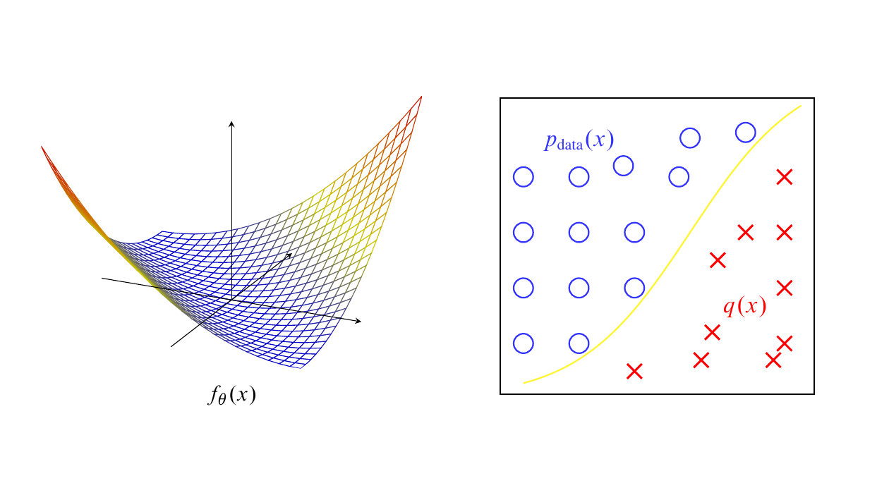
\[p_\theta(x) = \frac{e^{-f_\theta(x)}}{Z(\theta)}\]where $f_\theta(x)$ is the energy function, and
\[Z(\theta)=\int e^{-f_\theta(x)}dx\]is the normalizing constant. In language models like word2vec, the energy function may simply be the inner product of the input word vector with some context word vector, i.e. $f^c(w) = w\cdot c$, and the denominator is a sum over all words in the dictionary. In other applications, the energy function may be a neural network that maps input data to real valued numebers.
The density $p_\theta$ has high values on which the energy function $f_\theta$ has low values, so the landscape of the energy $f_\theta$ has low valleys along the data distribution and high hills outside the data distribution. Estimating an energy based model amounts to find ways to push down the energy function on the data manifold and push up elsewhere.
Performing Maximum Likelihood Estimation (MLE) or sampling requires computation of the constant $Z(\theta)$. However, for high dimensional data like languages and images, it is intractable to compute, and one has to rely on methods such as Langevin dynamics or Markov Chain Monte Carlo (MCMC) methods such as Hamiltonian Monte Carlo. The convergence of such methods may be slow, and may suffer especially if the dataset has multiple modes.
Derivation of the Method
NCE is a method to estimate energy based models that circumvents the need to compute the normalizing constant. The normalizing constant is treated as a trainable parameter, so that the model is specified as
\[\log p_\theta(x)= -f_\theta(x) - c\]where $c=\log Z(\theta)$. In this case, it is not possible to do MLE because one can simply drive the log density towards infinity by letting $c\to-\infty$.
Instead, the model is trained by doing a classification between the training data and some generated noises, in other words a (nonlinear) logistic regression. Label the training data as $\xi=1$ and label the noises as $\xi=0$. Let $q$ denote some noise distribution on the data space. Model $p(x\mid \xi=1)$ by $p_\theta(x)$ and model $p(x\mid \xi=0)$ by $q(x)$. Suppose the prior distribution of the labels is $p(\xi=1)=p(\xi=0)=1/2$, i.e., we assume equal amount of data and noise are supplied. Then using Bayes rule, the posterior of the class labels are:
- posterior of $\xi=1$ given $x\in\mathcal{X}$ from training dataset:
- posterior of $\xi=0$ given generated sample $\tilde{x}$:
Then, one can maximize the posterior log likelihood of training data \(\{x_i\}_{i=1}^n\) and noise \(\{\tilde{x}\}_{i=1}^n\) by maximizing the objective
where the expectations are approximated by sample means.
We generally have three requirements for the noise distribution $q$:
- the density function $q(x)$ is tractable to compute, so that it can be evaluated on any input $x$;
- we can easily obtain samples $\tilde{x}\sim q$ from the noise distribution;
- the support of $q$ should cover the support of data distribution, so in particular $q(x)\neq0$ for all $x$ such that $p_{\text{data}}(x)\neq 0$.
Typically, for simple tasks one could use Gaussian as the noise distribution. Besides the three requirements above, the noise distribution should not be too far away from the data distribution, otherwise the learning task is too easy and the energy model may not be able to learn anything meaningful. From the perspective of the energy landscape, NCE amounts to push up the energy landscape only at the specific locations of the noises. Thus, it would be useful for the noise mode to be close to the data mode (but may not necessary to be too close) so that learning can be more efficient.
Calculating the posteriors
In implementations, we often output log probabilities. We mention here an alternative formula for the two posteriors
\[r(x):=\frac{p_\theta(x)}{p_\theta(x)+q(x)}\]and
It is
\[r(x)=\sigma(\log p_\theta(x) - \log q(x)).\]where $\sigma$ is the sigmoid function. The derivation is as follows:
Implementation
See my github repo for an implementation of NCE on 2D data. Below are several examples. The left column shows samples from target data distributions, the middle column is the Gaussian noise, and the right column shows the estimated densities during training.


Cite as:
1
2
3
4
5
6
7
@article{lifei2022nce,
  title   = "Noise Contrastive Estimation",
  author  = "Li, Fei",
  journal = "https://lifeitech.github.io",
  year    = "2022",
  url     = "https://lifeitech.github.io/posts/nce/"
}
References
[1] M. Gutmann and A. Hyvärinen. “Noise-contrastive estimation: A new estimation principle for unnormalized statistical models”. Proceedings of the Thirteenth International Conference on Artificial Intelligence and Statistics. Vol. 9. Proceedings of Machine Learning Research. PMLR, 2010, pp. 297–304.
[2] Mnih, Andriy, and Yee Whye Teh. “A fast and simple algorithm for training neural probabilistic language models.” arXiv preprint arXiv:1206.6426 (2012).
Comments powered by Disqus.